Difference between revisions of "See the MRF development"
| Line 1: | Line 1: | ||
| − | Reynolds-Averaged Navier-Stokes formulation in the rotating frame. | + | The section describes the development for the Reynolds-Averaged Navier-Stokes formulation in the rotating frame. |
| − | + | To start, we will look at the acceleration term for a rotating frame around the z axis <math> (\vec \Omega)</math>. | |
Notation: I: inertial, R: rotating | Notation: I: inertial, R: rotating | ||
| − | + | For a general vector: | |
<math>\left [ \frac{d \vec A}{dt} \right ]_I = \left [ \frac{d \vec A}{dt} \right ]_R + \vec \Omega \times \vec A</math> | <math>\left [ \frac{d \vec A}{dt} \right ]_I = \left [ \frac{d \vec A}{dt} \right ]_R + \vec \Omega \times \vec A</math> | ||
| − | + | For the position vector: | |
<math>\left [ \frac{d \vec r}{dt} \right ]_I = \left [ \frac{d \vec r}{dt} \right ]_R + \vec \Omega \times \vec r</math> | <math>\left [ \frac{d \vec r}{dt} \right ]_I = \left [ \frac{d \vec r}{dt} \right ]_R + \vec \Omega \times \vec r</math> | ||
| Line 15: | Line 15: | ||
<math>\vec u_I = \vec u_R + \vec \Omega \times \vec r</math> | <math>\vec u_I = \vec u_R + \vec \Omega \times \vec r</math> | ||
| − | + | The acceleration is expressed as: | |
<math>\left [ \frac{d \vec u_I}{dt} \right ]_I = \left [ \frac{d \vec u_I}{dt} \right ]_R + \vec \Omega \times \vec u_I</math> | <math>\left [ \frac{d \vec u_I}{dt} \right ]_I = \left [ \frac{d \vec u_I}{dt} \right ]_R + \vec \Omega \times \vec u_I</math> | ||
| Line 25: | Line 25: | ||
<math>\left [ \frac{d \vec u_I}{dt} \right ]_I = \left [ \frac{d \vec u_R}{dt} \right ]_R + \frac{d \vec \Omega}{dt} \times \vec r + 2 \vec \Omega \times \vec u_R + \vec \Omega \times \vec \Omega \times \vec r</math> '''Eqn [1]''' | <math>\left [ \frac{d \vec u_I}{dt} \right ]_I = \left [ \frac{d \vec u_R}{dt} \right ]_R + \frac{d \vec \Omega}{dt} \times \vec r + 2 \vec \Omega \times \vec u_R + \vec \Omega \times \vec \Omega \times \vec r</math> '''Eqn [1]''' | ||
| − | Navier-Stokes equations in the inertial frame | + | The Navier-Stokes equations in the inertial frame are: |
<math> | <math> | ||
| Line 83: | Line 83: | ||
</math> | </math> | ||
| − | Eqn [ | + | Eqn [3] can be written as |
<math> | <math> | ||
| Line 92: | Line 92: | ||
</math> '''Eqn [5]''' | </math> '''Eqn [5]''' | ||
| − | Eqn [5] represents the Navier-Stokes equations in the rotating frame, in terms of | + | Eqn [5] represents the Navier-Stokes equations in the rotating frame, in terms of rotating velocities (convection velocity and convected velocity). |
Eqn [5] can be further developed so the convected velocity is the velocity in the inertial frame. | Eqn [5] can be further developed so the convected velocity is the velocity in the inertial frame. | ||
| Line 121: | Line 121: | ||
<math> | <math> | ||
\begin{cases} | \begin{cases} | ||
| − | \frac {\partial \vec u_R}{\partial t} + \frac{d \vec \Omega}{dt} \times \vec r + \nabla \cdot (\vec u_R \otimes \vec u_I) + \vec \Omega \times \vec u_I = - \nabla (p/\rho) + \nu \nabla \cdot \nabla (\vec | + | \frac {\partial \vec u_R}{\partial t} + \frac{d \vec \Omega}{dt} \times \vec r + \nabla \cdot (\vec u_R \otimes \vec u_I) + \vec \Omega \times \vec u_I = - \nabla (p/\rho) + \nu \nabla \cdot \nabla (\vec u_I) \\ |
\nabla \cdot \vec u_I = 0 | \nabla \cdot \vec u_I = 0 | ||
\end{cases} | \end{cases} | ||
| Line 157: | Line 157: | ||
| <math> | | <math> | ||
\begin{cases} | \begin{cases} | ||
| − | \nabla \cdot (\vec u_R \otimes \vec u_I) + \vec \Omega \times \vec u_I = - \nabla (p/\rho) + \nu \nabla \cdot \nabla (\vec | + | \nabla \cdot (\vec u_R \otimes \vec u_I) + \vec \Omega \times \vec u_I = - \nabla (p/\rho) + \nu \nabla \cdot \nabla (\vec u_I) \\ |
\nabla \cdot \vec u_I = 0 | \nabla \cdot \vec u_I = 0 | ||
\end{cases} | \end{cases} | ||
Revision as of 03:24, 27 May 2009
The section describes the development for the Reynolds-Averaged Navier-Stokes formulation in the rotating frame.
To start, we will look at the acceleration term for a rotating frame around the z axis  .
.
Notation: I: inertial, R: rotating
For a general vector:
![\left [ \frac{d \vec A}{dt} \right ]_I = \left [ \frac{d \vec A}{dt} \right ]_R + \vec \Omega \times \vec A](/images/math/d/d/7/dd7f88256c509a0be7a15c53f866d116.png)
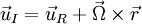
For the position vector:
![\left [ \frac{d \vec r}{dt} \right ]_I = \left [ \frac{d \vec r}{dt} \right ]_R + \vec \Omega \times \vec r](/images/math/4/1/3/4131b2e6b777a32980f1ba8735800c00.png)
The acceleration is expressed as:
![\left [ \frac{d \vec u_I}{dt} \right ]_I = \left [ \frac{d \vec u_I}{dt} \right ]_R + \vec \Omega \times \vec u_I](/images/math/7/f/2/7f20a49ddaaf0f5f75839a3418ed3021.png)
![\left [ \frac{d \vec u_I}{dt} \right ]_I = \left [ \frac{d \left [ \vec u_R + \vec\Omega \times \vec r \right ] }{dt} \right ]_R + \vec \Omega \times \left [ \vec u_R + \vec \Omega \times \vec r \right ]](/images/math/e/a/d/ead6fc46c5c666b0e14e890a9bca6578.png)
![\left [ \frac{d \vec u_I}{dt} \right ]_I = \left [ \frac{d \vec u_R}{dt} \right ]_R + \frac{d \vec \Omega}{dt} \times \vec r + \vec \Omega \times \underbrace{ \left [ \frac{d \vec r}{dt} \right ]_R }_{\vec u_R} + \vec \Omega \times \vec u_R + \vec \Omega \times \vec \Omega \times \vec r](/images/math/8/6/1/86139691a6747db6f2ccf1f4e78ed59a.png)
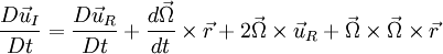
![\left [ \frac{d \vec u_I}{dt} \right ]_I = \left [ \frac{d \vec u_R}{dt} \right ]_R + \frac{d \vec \Omega}{dt} \times \vec r + 2 \vec \Omega \times \vec u_R + \vec \Omega \times \vec \Omega \times \vec r](/images/math/8/c/2/8c25e2e6b1588e6fb319dce79cabaddf.png) Eqn [1]
Eqn [1]
The Navier-Stokes equations in the inertial frame are:
 Eqn [2]
 Eqn [3]
Let's look at the left-hand side of the momentum equation of Eqn [2], by taking into account Eqn [1] for the acceleration term:

 Eqn [4]
since 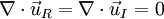
![\begin{alignat}{2}
\nabla \cdot \vec u_I & = \nabla \cdot \left [ \vec u_R + \vec \Omega \times \vec r \right ] = 0 \\
& = \nabla \cdot \vec u_R + \underbrace{\nabla \cdot \left [ \vec \Omega \times \vec r \right ]}_{0} = 0 \\
& = \nabla \cdot \vec u_R = 0
\end{alignat}](/images/math/b/2/d/b2dc4c3ad119b3f7f70bf2218afb73c0.png)
Also, it can be noted that
![\begin{alignat}{2}
\nabla \cdot \nabla (\vec u_I) & = \nabla \cdot \nabla \left [ \vec u_R + \vec \Omega \times \vec r \right ] \\
& = \nabla \cdot \nabla (\vec u_R) + \nabla \cdot \underbrace{\nabla (\Omega \times \vec r)}_{0} \\
& = \nabla \cdot \nabla (\vec u_R )
\end{alignat}](/images/math/5/b/c/5bc95681ab4a1cdaff6042763b45fcd7.png)
Eqn [3] can be written as
 Eqn [5]
Eqn [5] represents the Navier-Stokes equations in the rotating frame, in terms of rotating velocities (convection velocity and convected velocity).
Eqn [5] can be further developed so the convected velocity is the velocity in the inertial frame.
The term 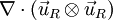 can be developed as:
![\begin{alignat}{2}
\nabla \cdot (\vec u_R \otimes \vec u_R) & = \nabla \cdot ( \vec u_R \otimes \left [ \vec u_I - \vec \Omega \times \vec r \right ] ) \\
& = \nabla \cdot (\vec u_R \otimes \vec u_I) - \underbrace{\nabla \cdot \vec u_R}_{0} (\vec \Omega \times \vec r) - \underbrace{\vec u_R \cdot \nabla(\vec \Omega \times \vec r)}_{\vec \Omega \times \vec u_R} \\
& = \nabla \cdot (\vec u_R \otimes \vec u_I) - \vec \Omega \times \vec u_R
\end{alignat}](/images/math/2/a/1/2a1085f93629d5eab99efa8979e5b362.png)
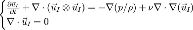
So, the steady term of left-hand side of Eqn [5] can be written as
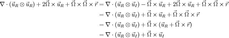
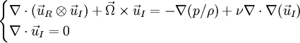
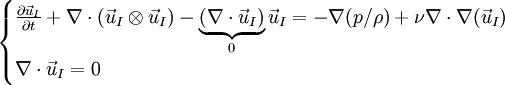
Eqn [5] can be written in terms of the absolute velocity:
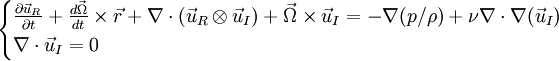 Eqn [6]
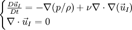
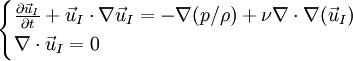
In summary, for multiple frames of reference, the Reynolds-averaged Navier-Stokes equations for steady flow can be written
Frame Convected velocity RANS equations Inertial absolute velocity 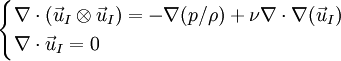
Rotating relative velocity 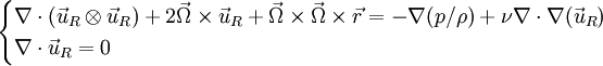
Rotating absolute velocity